Ensemble Models and Outlook

20. Ensemble Models and Outlook#

In the past chapters, several common machine learning algorithms were introduced. They come with different strengths and weaknesses. And, although the code execution always looks very similar, they all require different parameters and adjustments.

Before we move on to the next topic, let us introduce a very generally applicable trick in machine learning: ensemble learning.

Ensemble learning is a method where multiple models are trained and combined to solve the same problem. The key idea is that by combining multiple models, we can achieve better performance than any single model alone. This idea is simple, yet in practice, ensemble models are surprisingly effective. There are two main types of ensemble methods: bagging and boosting.

We will first look at the general idea behind bagging and later apply some common strategies to the data from the last chapter on predicting obesity levels.

20.1. Many trees know more than a single tree#

For illustrative purposes, we best start with two-dimensional data. The following dummy data contains data points from two classes and follows a spiral pattern.

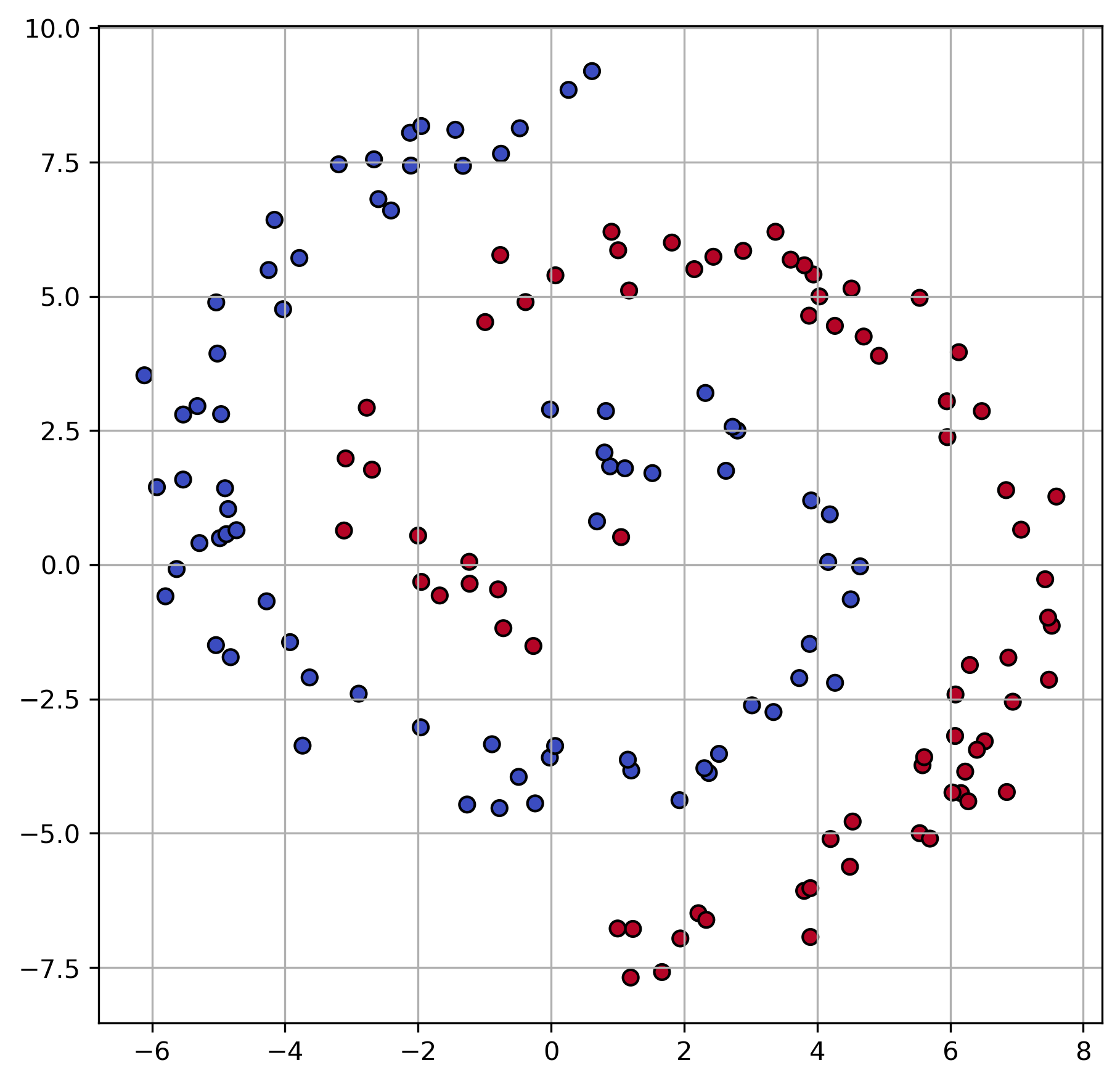
../_images/eb2f214e7e02f11cea27f8b50be59983d8fea2ba287bd652d64021df8d6fbc00.png

A decision tree can handle such data, but the highly non-linear arrangement of the data points makes it slightly cumbersome for such a model. The decision tree (Section 18) learns decision boundaries along the x- and y-axis, and the shape of a spiral cannot be approximated very well with only a few such binary decisions.

Let us train two decision trees, one with small max_depth, and one without any depth restrictions:

from sklearn.tree import DecisionTreeClassifier

depth1, depth2 = 4, None
tree1 = DecisionTreeClassifier(max_depth=depth1,
                              random_state=0)
tree2 = DecisionTreeClassifier(max_depth=depth2,
                              random_state=0)
# Train the decision trees
tree1.fit(X, y)
tree2.fit(X, y)

DecisionTreeClassifier(random_state=0)

In a Jupyter environment, please rerun this cell to show the HTML representation or trust the notebook.
On GitHub, the HTML representation is unable to render, please try loading this page with nbviewer.org.

We can have both decision trees making predictions on a regular x-y grid of points to display which regions will receive the label 0 (blue) or 1 (red).

Text(0.5, 1.0, 'Tree with max_depth None')

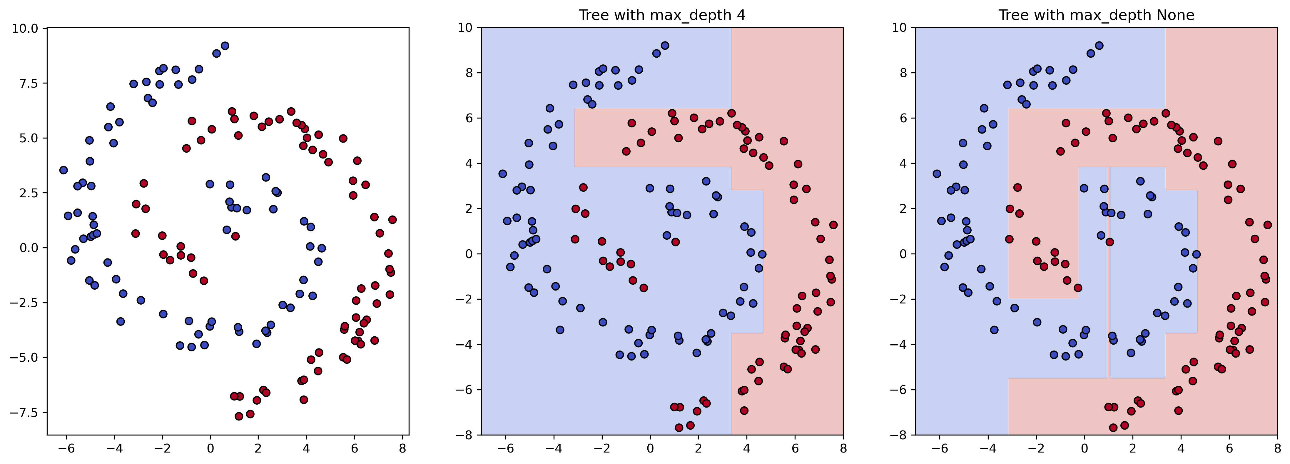
../_images/03b649db72d0c24bc1ccbd0212412265d56b67cd3d269bc6683efa39f427b4a8.png

As expected, the decision tree with low depth is incapable of modeling the data’s spiral shape very well. This is also called underfitting. On the other hand, the tree with unrestricted depth will come with the problem of overfitting.

Finding a good sweet spot between under- and over-fitting can be difficult for decision trees. It is usually much more effective to rather combine many trees to form an ensemble model. Two key concepts for training an ensemble model are: bagging and boosting [Kotsiantis, 2011].

20.2. Bagging (Bootstrap Aggregating)#

Bagging is a technique that involves training multiple models on different subsets of the training data and then combining their predictions [Breiman, 1996]. Each subset is created by randomly sampling the training data with replacement (bootstrap sampling). The final prediction is usually obtained by averaging the predictions (for regression) or taking a majority vote (for classification).

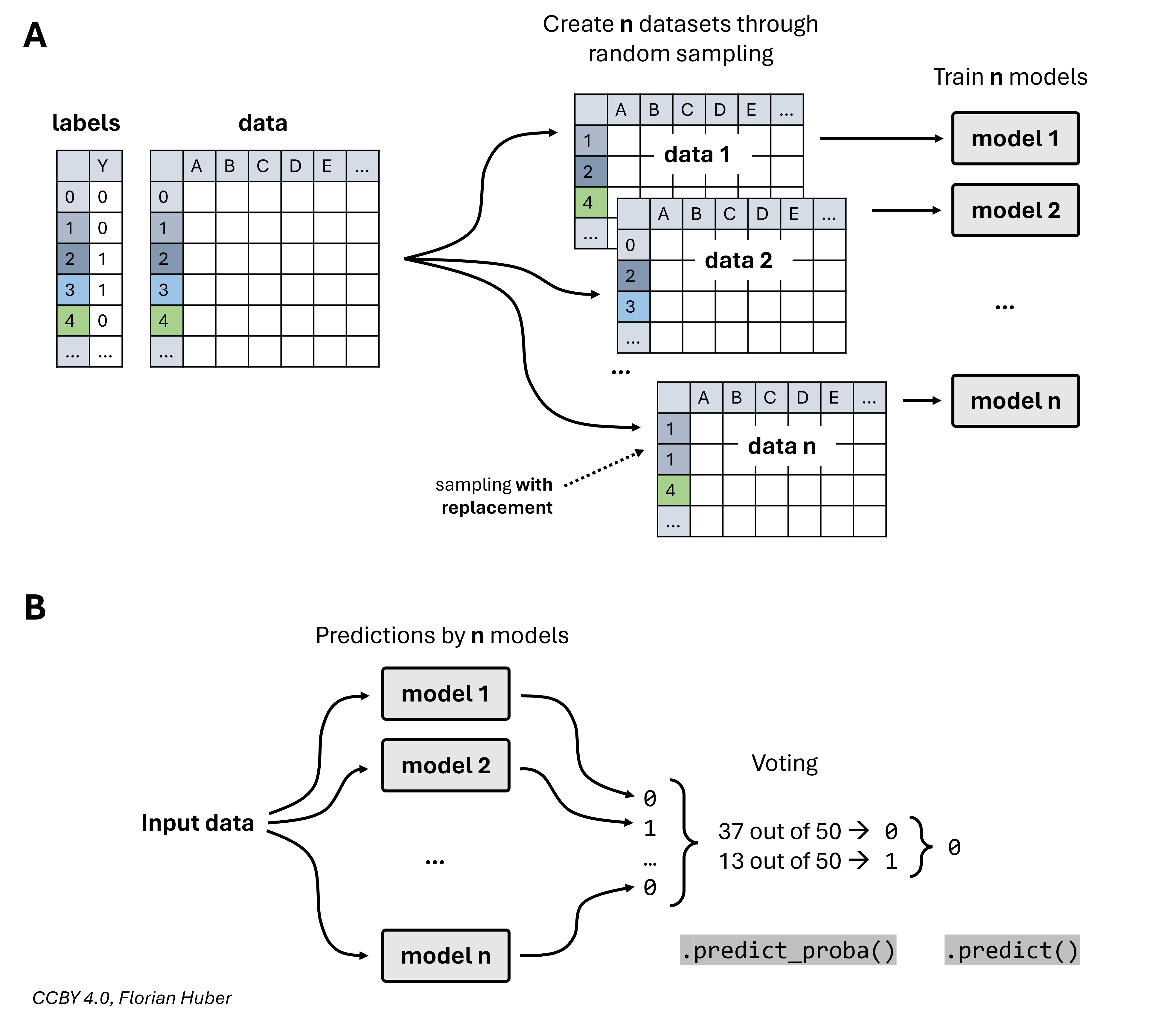
../_images/fig_ensemble_bagging.png — Fig. 20.1 In the bagging approach, the training data is randomly sampled (usually with replacement) \(n\) times to then train \(n\) models (A). During prediction, the output of all \(n\) models is counted and the final predictions is defined by voting (B).#

The most common example of such an ensemble model is the Random Forest.

20.2.1. Many Trees are a Forest: Random Forest#

Random Forest is an ensemble method that combines multiple decision trees using bagging and random feature selection. Each tree is trained on a different bootstrap sample of the data, and a random subset of features is used for splitting nodes. The final prediction is made by averaging the predictions of all individual trees (for regression) or by majority voting (for classification).

To better understand how (and why) this works, we can create our own simple version of such a bagging algorithm:

# Combine all trees
class SimpleBagging:
    def __init__(self, trees):
        self.trees = trees

    def predict_proba(self, x):
        predictions = np.array([t.predict(x) for t in self.trees])
        return np.mean(predictions, axis=0)

Let us now train 15 decision trees and combine their result in the end.

Please try the following code also with BOOTSTRAP = False and see if you understand what happens.

MAX_DEPTH = 5
BOOTSTRAP = True

# Train 15 decision trees
trees = []
rng = np.random.default_rng(seed=0)
for _ in range(15):
    if BOOTSTRAP:
        idx = rng.choice(np.arange(NUM_POINTS), NUM_POINTS)
    else:
        idx = np.arange(NUM_POINTS)
    X_bootstrap = X[idx]
    y_bootstrap = y[idx]
    tree = DecisionTreeClassifier(max_depth=MAX_DEPTH, random_state=0)
    trees.append(tree.fit(X_bootstrap, y_bootstrap))

# Combine the trees
bagging_clf = SimpleBagging(trees)

We can again use the grid of x-y points to show the decision boundaries of all 15 trees as well as the ensemble model:

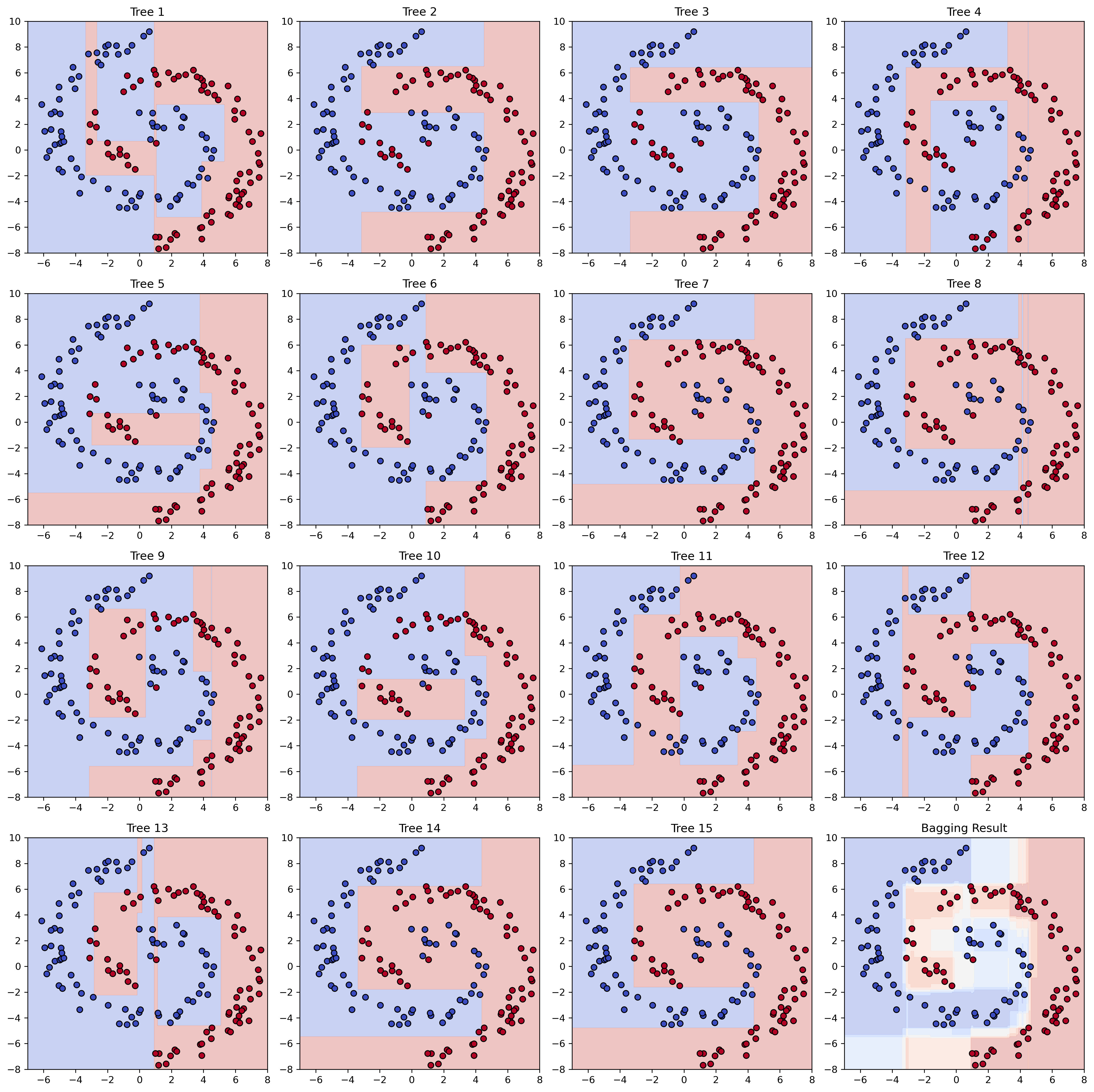
../_images/91d6c2c2f1cca81993fc6889e68693273419855466d303845ec99d724b0cfef9.png

The individual decision trees were trained with different subsets of our data (for BOOTSTRAP = True). As a consequence, they all learned different decision boundaries, none of them being very good overall due to the limited depth of each tree.

The ensemble model, however, generally performs much better. It also allows us to gain more than just a binary class prediction: we can get the fraction of trees voting for or against a certain class which can give us a sense of uncertainty of the model prediction. In practice, this is often used to further rate or filter model predictions.

20.3. Use-case: Obesity-Level Prediction#

Moving away from the illustrative two dimensional toy data, we can apply the same idea to the data set from the last chapter to predict obesity levels.

/tmp/ipykernel_3010/166062201.py:6: FutureWarning: Downcasting behavior in `replace` is deprecated and will be removed in a future version. To retain the old behavior, explicitly call `result.infer_objects(copy=False)`. To opt-in to the future behavior, set `pd.set_option('future.no_silent_downcasting', True)`
  data[binary_columns] = data[binary_columns].replace({'no': 0, 'yes': 1})

	Age	Height	Weight	family_history_with_overweight	FCVC	NCP	SMOKE	CH2O	SCC	...	CAEC_no	CALC_Always	CALC_Frequently	CALC_Sometimes	CALC_no	MTRANS_Automobile	MTRANS_Bike	MTRANS_Motorbike	MTRANS_Public_Transportation	MTRANS_Walking
0	21.0	1.62	64.0	1	2.0	3.0	0	2.0	0	...	False	False	False	False	True	False	False	False	True	False
1	21.0	1.52	56.0	1	3.0	3.0	1	3.0	1	...	False	False	False	True	False	False	False	False	True	False
2	23.0	1.80	77.0	1	2.0	3.0	0	2.0	0	...	False	False	True	False	False	False	False	False	True	False
3	27.0	1.80	87.0	0	3.0	3.0	0	2.0	0	...	False	False	True	False	False	False	False	False	False	True
4	22.0	1.78	89.8	0	2.0	1.0	0	2.0	0	...	False	False	False	True	False	False	False	False	True	False

5 rows × 26 columns

from sklearn.model_selection import train_test_split

# Split data into training and testing sets
X_train, X_test, y_train, y_test = train_test_split(X, y, test_size=0.3, random_state=42)

20.3.1. Single Decision Tree#

Let’s start again with a single decision tree, here with a set max_depth. As we saw in the last chapter, such a model works OK-ish on this dataset.

from sklearn.tree import DecisionTreeClassifier
from sklearn.metrics import accuracy_score

# Initialize base classifier
tree = DecisionTreeClassifier(max_depth=6)
tree.fit(X_train, y_train)

# Make predictions
y_pred = tree.predict(X_test)

# Evaluate the model
accuracy = accuracy_score(y_test, y_pred)
print(f'Accuracy of Decision Tree Classifier: {accuracy:.2f}')

Accuracy of Decision Tree Classifier: 0.86

We do not have to build our own class for combining multiple decision trees as we did above with the spiral example. We can simply implement this via the Scikit-Learn BaggingClassifier class:

from sklearn.ensemble import BaggingClassifier

# Initialize base classifier
base_clf = DecisionTreeClassifier(max_depth=6)

# Initialize bagging classifier
bagging_clf = BaggingClassifier(estimator=base_clf, n_estimators=50, random_state=42)

# Train the bagging classifier
bagging_clf.fit(X_train, y_train)

# Make predictions
y_pred = bagging_clf.predict(X_test)

# Evaluate the model
accuracy = accuracy_score(y_test, y_pred)
print(f'Accuracy of Bagging Classifier: {accuracy:.2f}')

Accuracy of Bagging Classifier: 0.89

However, the Random Forest is famous enough to be implemented already in Scikit Learn:

from sklearn.ensemble import RandomForestClassifier

# Initialize Random Forest classifier
rf_clf = RandomForestClassifier(max_depth=6, n_estimators=50, random_state=42)

# Train the Random Forest classifier
rf_clf.fit(X_train, y_train)

# Make predictions
y_pred = rf_clf.predict(X_test)

# Evaluate the model
accuracy = accuracy_score(y_test, y_pred)
print(f'Accuracy of Random Forest Classifier: {accuracy:.2f}')

Accuracy of Random Forest Classifier: 0.89

20.4. Boosting#

Boosting is another ensemble technique that focuses on training models sequentially. Each new model attempts to correct the errors made by the previous ones. This way, the models “boost” the performance by focusing more on the difficult cases.

There are several different boosting techniques and strategies [Tanha et al., 2020, Bentéjac et al., 2021]. In AdaBoost, for instance, each data point is assigned a weight. Initially, every example starts with the same weight. Then, iteratively, the weights are adjusted depending on the prediction errors with weights increasing for misclassified data points [Freund and Schapire, 1997], see also Fig. 20.2.

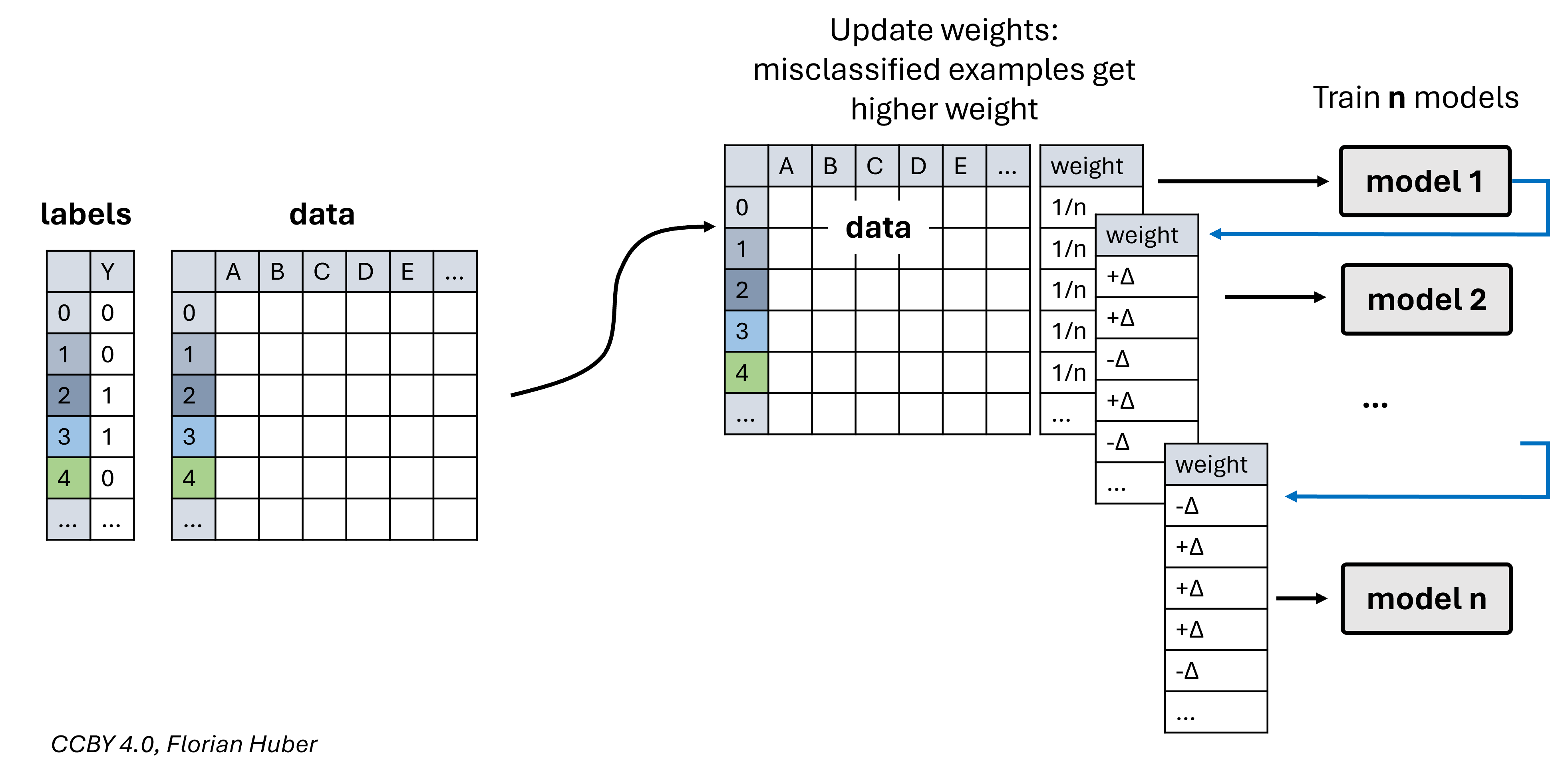
../_images/fig_ensemble_boosting.png — Fig. 20.2 In the boosting approach (e.g. AdaBoost), the \(n\) models are trained iteratively and not in parallel (as it is done in bagging). The training of a model depends on the prediction error of the former model. In AdaBoost, for instance, each data point starts with the same weight. Then, weights are adapted based on the model outcome with increasing weights for misclassifications.#

A very successful other group of boosting techniques (at least for things like Kaggle challenges) are gradient boosting algorithms such as “XGBoost” or “LightGBM”. For an in depth overview on gradient boosting, see [Bentéjac et al., 2021].

from sklearn.ensemble import AdaBoostClassifier

# Initialize base classifier
base_clf = DecisionTreeClassifier(max_depth=6)

# Initialize AdaBoost classifier
ada_clf = AdaBoostClassifier(estimator=base_clf, n_estimators=50, random_state=42)

# Train the AdaBoost classifier
ada_clf.fit(X_train, y_train)

# Make predictions
y_pred = ada_clf.predict(X_test)

# Evaluate the model
accuracy = accuracy_score(y_test, y_pred)
print(f'Accuracy of AdaBoost Classifier: {accuracy:.2f}')

/home/runner/micromamba/envs/data_science/lib/python3.12/site-packages/sklearn/ensemble/_weight_boosting.py:527: FutureWarning: The SAMME.R algorithm (the default) is deprecated and will be removed in 1.6. Use the SAMME algorithm to circumvent this warning.
  warnings.warn(

Accuracy of AdaBoost Classifier: 0.97

With some more parameters searches we can probably improve even a little more… (try it out yourself!).

base_clf = DecisionTreeClassifier(max_depth=10)
ada_clf = AdaBoostClassifier(estimator=base_clf, n_estimators=200, random_state=42)
ada_clf.fit(X_train, y_train)

y_pred = ada_clf.predict(X_test)

# Evaluate the model
accuracy = accuracy_score(y_test, y_pred)
print(f'Accuracy of AdaBoost Classifier: {accuracy:.2f}')

/home/runner/micromamba/envs/data_science/lib/python3.12/site-packages/sklearn/ensemble/_weight_boosting.py:527: FutureWarning: The SAMME.R algorithm (the default) is deprecated and will be removed in 1.6. Use the SAMME algorithm to circumvent this warning.
  warnings.warn(

Accuracy of AdaBoost Classifier: 0.97

The accuracy looks promising, but let’s better also check the confusion matrix.

from sklearn.metrics import confusion_matrix

fig, ax = plt.subplots(figsize=(7, 7), dpi=300)

sb.heatmap(confusion_matrix(y_test, y_pred),
           annot=True, cmap="Blues", cbar=False, fmt=".0f",
           xticklabels=ada_clf.classes_,
           yticklabels=ada_clf.classes_)
ax.set_xlabel("True label", fontsize=14)
ax.set_ylabel("Predicted label", fontsize=14)
plt.show()

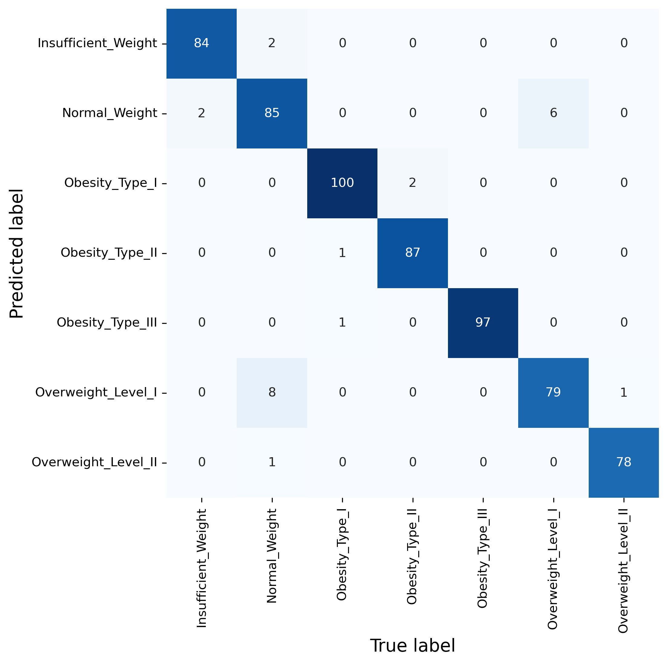
../_images/b956810855a277adaa640043a2b03c00a457d798d3059e43a33b13297de82394.png

In many cases, ensemble models outperform individual models when it comes to robustness and the quality of the predictions. They come with two downsides. Firstly, they require the training and internal handling of dozens or hundreds of models instead of only one. For moderately sized datasets this is usually a price people are very willing to pay.

Secondly, ensemble models are often harder to interpret. An individual decision tree is, in principle, fully human-readable. However, a random forest of hundreds of trees is not as easily accessible. There are techniques that help us to interpret predictions of such ensemble models, such as SHAP [Lundberg and Lee, 2017] [Lundberg et al., 2020]. Feel free to explore those tools yourself (e.g. SHAP).

20.5. Outlook: More on Machine Learning#

This course is meant as a general introduction to data science. Machine Learning is, no doubt, one of the most essential tools for any data scientist. In fact, it is not just one tool but rather an entire toolbox full of very powerful methods. While nobody will be able to be on top of all possible tools in this toolbox, having at least an intuitive understanding of the most prominent types of tools is key for modern data science workflows. This includes unsupervised methods such as clustering techniques and dimensionality reduction, as well as supervised methods like k-nearest neighbors, linear regression, or decision trees.

We have covered those techniques in this and the prior chapters with exactly this goal in mind. The focus was on a basic intuition and first application of these methods. You will hopefully later realize, that many core concepts apply to other machine learning approaches, too. Still, the extend of machine learning covered in this book is mostly supposed to serve as a good first basis. When you face actual problems that you want to solve using machine learning, you will probably have to expand this basis quiet a bit. Here, we did not cover all algorithms in full depth. And we also had to leave out several common limitations and pitfalls. And, as you probably already know, there are many machine learning techniques beyond the ones introduced in the prior chapters, from support vector machines all the way to modern deep learning approaches.

While we cannot (or do not want) to cover all those techniques in this introduction to data science, there are -luckily- many good resources to help you deepen your understanding of individual methods and broaden your knowledge on various techniques. This includes the large field of deep learning, which is highly relevant for many data science applications, but also something that requires a substantial investment of time to master.

20.5.1. Further Learning Resources#

Online courses and tutorials:
There are many, in fact probably too many, courses and tutorials out there. One of them that is clearly a long time recommendation is Andrew Ng’s open online courses such as the Machine Learning Introduction on coursera.

Books on Machine Learning and Deep Learning:

“Machine Learning with PyTorch and Scikit-Learn: Develop machine learning and deep learning models with Python” [Raschka et al., 2022]
“Understanding Deep Learning” by Simon Prince, MIT Press, 2023 [Prince, 2023]
“Introduction to pytorch”, [Ketkar et al., 2021]

By continuing to explore these resources, you can build a solid foundation in machine learning and stay up-to-date with the latest advancements in the field.

Happy (machine) learning!