15. Supervised Machine Learning - Introduction

15.1. What is Machine Learning?

There is still a lot of confusion about terms like artificial intelligence (or: A.I.), machine learning, and deep learning. The aim of this course is not to give a full in-depth introduction to all those topics, because this clearly demands one (or usually: multiple) course on its own. For more in-depth information we will provide some resources at the end of this chapter.

However, what this section should show is, that the underlying idea of machine learning is often quite approachable. And some of the respective techniques can be used with relative ease, at least from the code perspective. If you haven’t learned the basics of machine learning before, it is unlikely that this section will make you feel like you have mastered the art. But, again, this is not the main goal.

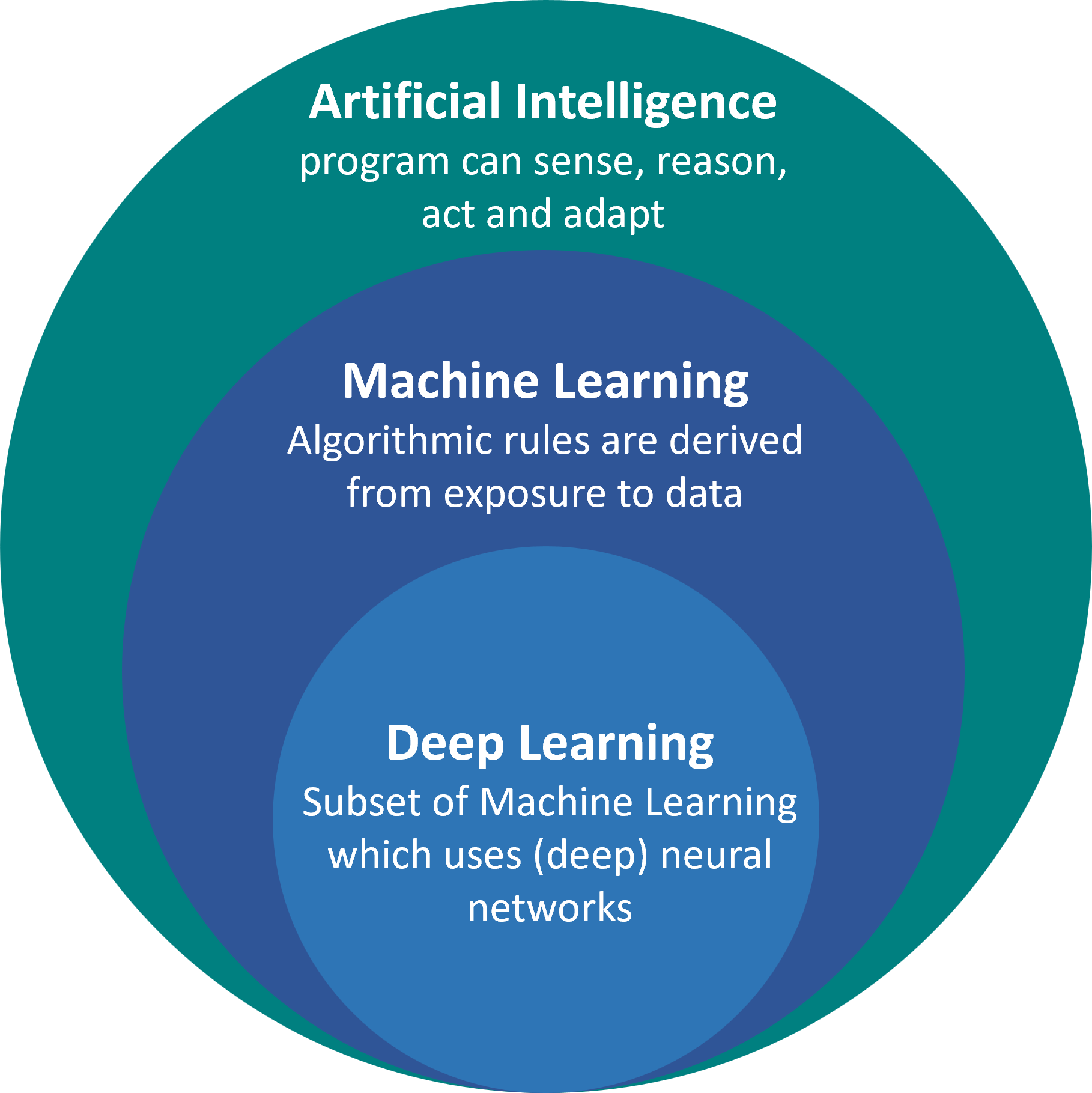
Machine learning is a subfield of artificial intelligence (see Fig. 14.1), which often makes this sound very intimidating at first. In its full complexity, this is indeed hard to master. But it is important to note at this point, that machine learning itself can also be seen as just another tool that we have as data scientists. In fact, many of its techniques are no more complicated or complex than methods in dimensionality reduction or clustering that we have seen in the last chapters (actually, those are often considered machine learning techniques as well, but we will skip this discussion for now).

Fig. 15.1 Machine Learning is a field of techniques that belongs to artificial intelligence. Currently, machine learning is even the main representation of artificial intelligence with deep learning being the most prominent subset. Here, however, we will focus on more classical machine learning techniques (no worries, those remain equally important in real-life practice!).

The key idea behind machine learning is that we use algorithms that “learn from data”. Learning here is nothing magic and typically means something very different from our everyday use of the word “learning” in a human context. Learning here simply means that the rules by which a program decides on its outcome or behavior are no longer hard-coded by a person, but they are automatically searched and optimized.

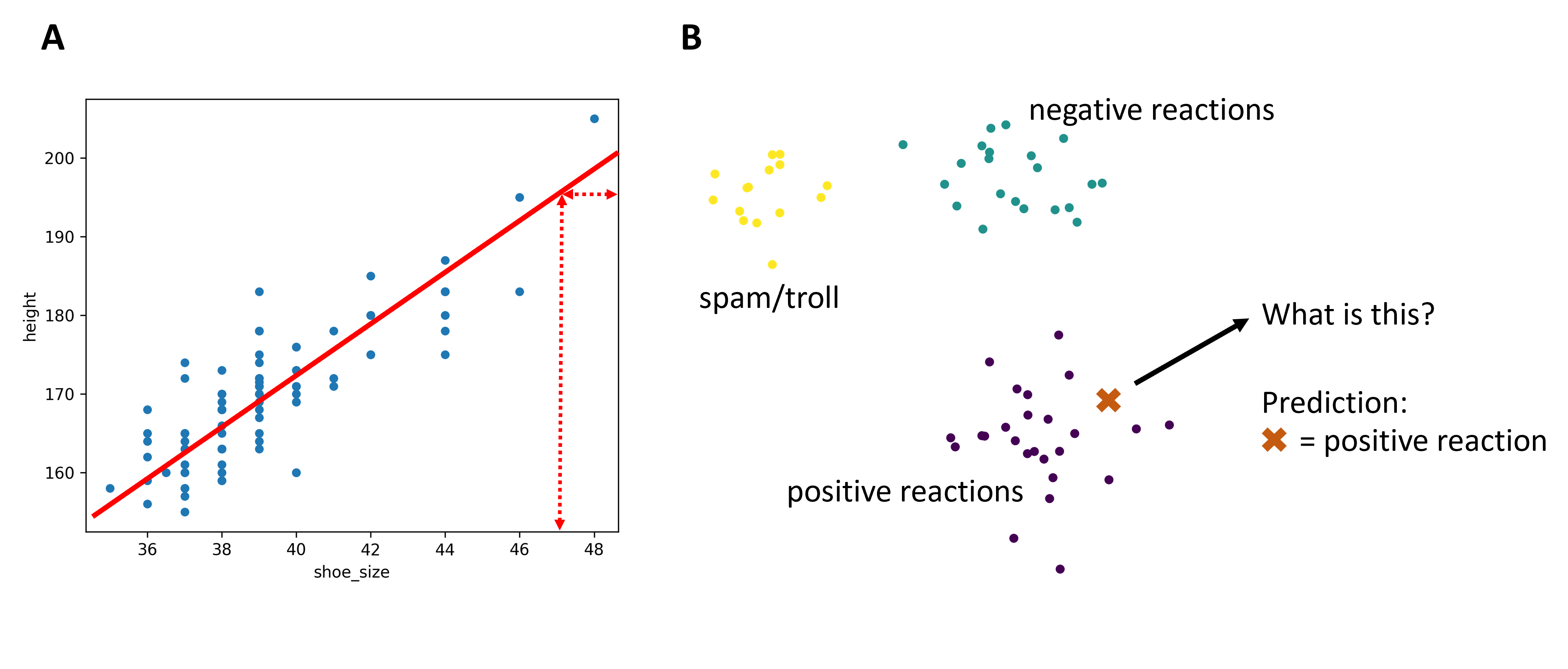
To give you an idea of how simple this “learning” can be: Imagine we have two highly correlated features, for instance the shoe size and the height of of many people. We could than automatically find a good linear fit function and then use this to make predictions for new data entries. Say, you find footprints of size 47 after a robery, then your new “machine learning model” (yes, that’s simply the linear fit!) can predict the height of that person (Fig. 15.2A). The prediction is probably not perfect, but we have good reasons to believe that it most likely won’t be too far off either.

Or, think of several chat messages that we clustered into “spam”, “negative”, and “positive” and which is nicely reflected by their position in a 2D plot after dimensionality reduction (Fig. 15.2B). If we now receive a new message which ends up clearly within the “positive” cluster, then we can obviously risk the first best guess of saying that this might be a positive message as well. Again, we could be wrong, but based on the data we have, this simply seems to be the best guess we can do.

So, when is this going to be called machine learning? When we have an algorithm that does this guessing based on the data for us it is machine learning. If we do the guessing, it is not machine learning.

Fig. 15.2 Even before coming to this chapter, we have already worked with techniques that would actually allow to make predictions on the basis of known data points. A, when we looked at (high) correlations this already implied that there is a more or less reliable link between different features. B, when we think of clustering and dimensionality reduction it seems rather obvious that we could make predictions for new datapoints based on their lower dimensional position!

Before we look at some actual machine learning techniques, a few key terms and distinctions should be explained.

15.1.1. Supervised vs. Unsupervised Learning

In machine learning, we distinguish supervised learning and unsupervised learning.

Supervised Learning involves training a model on a labeled dataset, which means that each training example is paired with an output label. The model learns to make predictions based on this input-output mapping. Common tasks in supervised learning include classification and regression. An example of supervised learning is spam email detection, where the model is trained on emails labeled as “spam” or “not spam.”

Unsupervised Learning, on the other hand, involves training a model on data that does not have labeled responses. The goal here is to infer the natural structure present within a set of data points. This is often used for clustering and association problems. An example of unsupervised learning is customer segmentation, where the model identifies distinct groups of customers based on purchasing behavior without prior knowledge of the group definitions.

Wait. That sounds familiar, right?
And indeed, this is exactly what we covered in the prior sections! Many algorithms used in dimensionality reduction (Section 14) and clustering (Section 12) were already machine learning and examples of unsupervised learning.

15.1.2. Classification vs. Regression

In machine learning, we distinguish two types of tasks that a model can perform: classification and regression.

Classification means that models will predict the class of unknown data points based on what they “learned” from labeled data. Labeled data means that this is data for which we know the true labels (also called: targets or ground truth). For example, in a medical diagnosis application, a classification model might predict whether a patient has a particular disease (e.g., positive or negative) based on their medical records.

Regression means that models will predict one (or multiple) numerical values for unknown data points. For instance, a regression model could predict house prices based on features like size, location, and the number of bedrooms. Unlike classification, where the output is a discrete class, regression outputs continuous values.

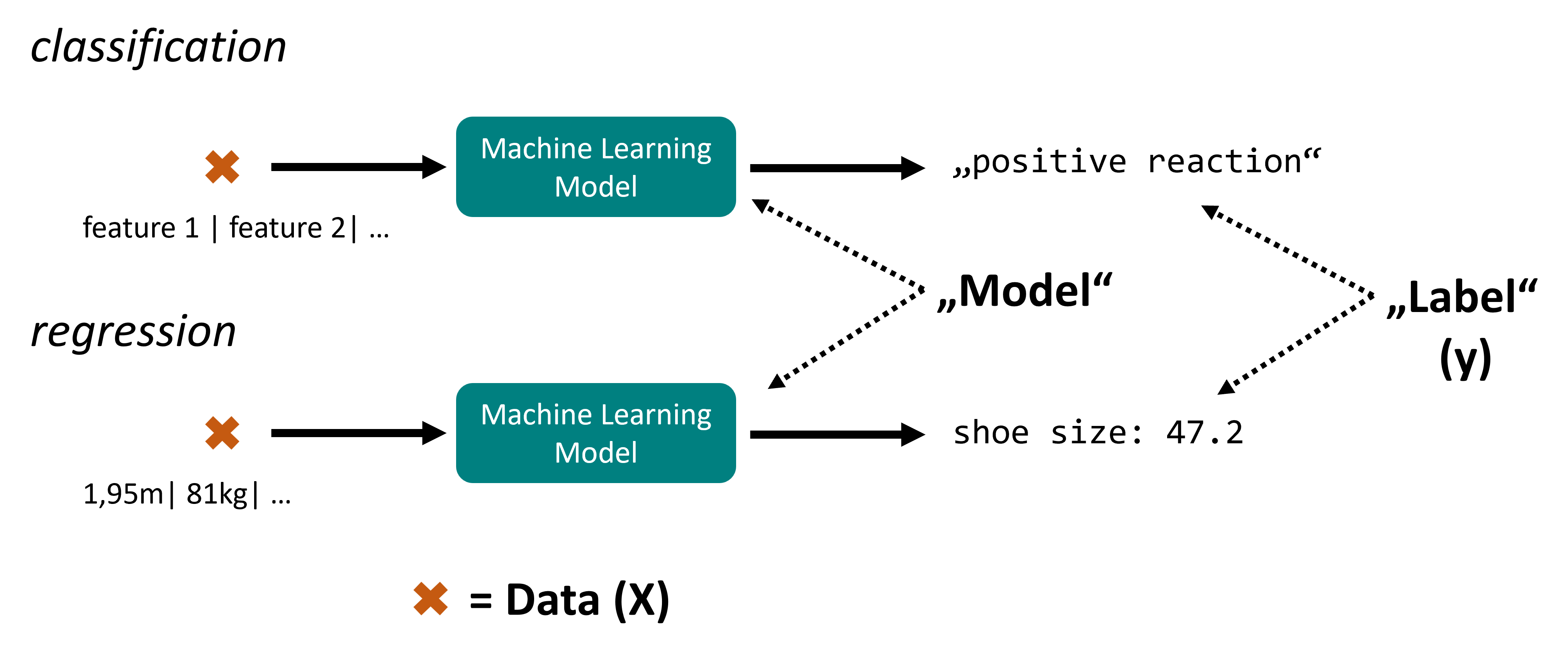
Both classification and regression fall under the category of supervised learning because they require labeled training data. An illustration of this distinction can be seen in Fig. 15.3, where one side shows the discrete class predictions of a classification task and the other shows the continuous value predictions of a regression task.

Fig. 15.3 In machine learning we distinguish classification and regression tasks. The key difference is that classification models will predict one out of several possible categories while regression models output numerical values (floats).

15.1.3. Features and Labels

Features are the input variables used to make predictions. Labels are the output variable that the model is trying to predict. For example, in a dataset of house prices, features might include the size of the house, the number of bedrooms, and the neighborhood, while the label would be the price of the house.

15.2. Training & Testing

For the following sections, we need a few more key terms:

• model: you can think of a machine learning model as a program function. It takes a certain, well-defined input (the data, often lazyly written as \(X\)) and generates predictions or labels (lazyly written: \(y\)).

• A model is trained on data with known labels. This is what is meant by the word learning in machine learning. However, this learning has little to no resemblance to human learning. It usually refers to an automated optimization on a given target which is expressed in terms of maths.

• What is automatically optimized in the model training are the model parameters. Those are thereby “learned” by the model during training. This is different from general model settings that are called hyperparameters and have to be set by us (or, they are pre-defined as default values by the code developers).

• The prediction of labels is called prediction or inference. This should happen after the model training.

15.2.1. How do we know how good our model is?

The tricky part about applying supervised machine learning models is that we train the model using (more or less-) well-understood data and later want to use its predictions on unknown data. So, we want to use our model for data where we don’t know the correct labels ourselves (say, predicting tomorrow’s weather). Or, we could know the labels but do not want to manually create those for all cases (for instance: classify all incoming mail as spam or no-spam).

But, can we really trust the model’s predictions?

As the name says, everything the model outputs are predictions. For all models we will consider here, every single model output is uncertain and could be wrong. With the tools we have at hand in this section, we cannot even estimate the chance of failing. But, we can measure how reliable our model is on average!

For this, we need to do the single most important action in machine learning,: the train/test split.

15.2.2. Train/Test split

For supervised machine learning, we need data (\(X\)) and corresponding labels (\(y\)). To avoid blindly applying our model to truly unseen and unknown data, we virtually always split our data into training and test data. As the name suggests, the training data can be used to train our machine learning model. The test data is kept and will never be used in training, but only to assess the quality of predictions of our model. Typically, we want as much data as possible for the training since more data usually correlates with better models. However, we also have to reserve enough data for the test set to later guarantee a meaningful assessment of our model.

We will later see that this can easily be done by using the train_test_split function from Scikit-Learn. Scikit-Learn is the main Python library for machine learning methods that are not deep learning [Pedregosa et al., 2011] and we will use this throughout the following chapters.