9. Data Pre-Processing#
9.1. What is Data Pre-Processing?#
We have now arrived what we called Scrub Data in the ASEMIC data science workflow. More formally, this is usually termed Data Pre-Processing and is a crucial step in every data science project. This process involves the preparation and cleansing of raw data to make it suitable for further analysis and modeling. In essence, data pre-processing is about transforming raw data into a clean dataset that is free from errors, inconsistencies, and is formatted appropriately for use in analytics applications.
The necessity for data pre-processing arises from the fact that real-world data is often incomplete, inconsistent, and/or lacking in certain behaviors or trends. Data might also be contaminated by errors or outliers that could potentially skew the results of any analysis performed.
9.1.1. Why is it Important?#
An often-heard quote in data science, most frequently in machine learning, is:
Garbage in, garbage out!
This phrase underscores a crucial truth about data science: the quality of the output is heavily dependent on the quality of the input. With a huge range of sophisticated tools and techniques available today, there is a common misconception that these tools can automatically correct or overcome shortcomings in the data. While modern technologies such as machine learning and artificial intelligence are powerful in extracting patterns and making predictions, they are not capable of performing miracles. Poor-quality data will likely result in poor-quality insights, leading to decisions that could be misleading or even detrimental.
Therefore, investing time in data pre-processing not only enhances the reliability of your data but also significantly boosts the effectiveness of the analytical models that process this data. This step ensures that subsequent analyses are both accurate and robust, providing meaningful insights that are based on a solid foundation of clean and well-structured data.
Data pre-processing is usually perceived as a much less “shiny” part of a data science process when compared to more “fancy” steps such as data visualization or training a machine learning model. It is not uncommon though, that the data acquisition and data preparation phase is what ultimately determines if a project will be a huge success or a failure!
9.1.2. Steps in Data Pre-Processing#
The process of data pre-processing includes several key steps:
Handling Missing Data: Filling or removing data entries that are missing to prevent errors in analysis.
Data Integration: Combining data from multiple sources to create a comprehensive dataset.
Data Transformation: Normalizing, scaling, or converting data to ensure that the dataset has a consistent scale and format.
Data Cleaning: Removing noise and correcting inconsistencies, which may involve addressing outliers, duplicate data, and correcting typos.
Data Reduction: Reducing the complexity of data, which can involve decreasing the number of features in a dataset or modifying the dataset to focus on important attributes.
These steps help in transforming raw data into a refined format that enhances the analytical capabilities of data science tools, leading to more accurate and insightful outcomes.
9.2. Dealing with Missing Values#
9.2.1. Understanding Missing Values#
Missing data is a prevalent issue in most data-gathering processes. It can occur for a variety of reasons including errors in data entry, failures in data collection processes, or during data transmission. The presence of missing values can significantly impact the performance of data analysis models, as most algorithms are designed to handle complete datasets.
Handling missing data is therefore a crucial step; if not addressed properly, it can lead to biased or invalid results. Different strategies can be employed depending on the nature of the data and the intended analysis.
9.2.2. Techniques to Handle Missing Values#
9.2.2.1. 1. Deletion#
Listwise Deletion: This involves removing any data entries that contain a missing value. While straightforward, this method can lead to a significant reduction in data size, which might not be ideal for statistical analysis.
Pairwise Deletion: Used primarily in statistical analyses, this method only excludes missing data in calculations where it is relevant. This allows for the use of all available data, although it can complicate the analysis process.
9.2.2.2. 2. Imputation#
Imputation means that we try to make good guesses of what the missing data could have been. It therefore is about much more than just spending a bit more time compared to a simple deletion step. Whether or not it is appropriate to use imputation depends on how well we understand the data and how sensitive the following data science tasks are. Suppose we, or the experts we collaborate with, do not have a very solid understanding of the data, its meaning, its measurement process etc.. In that case, we should usually not include imputation because it comes with a very high risk of introducing artifacts that we are not aware of.
The same is true if the following analysis is very sensible and thus requires properly measured values.
In other cases, however, imputation can indeed improve later results because it might allow us to work with a larger part of the available data. Common imputation types are:
Mean/Median/Mode Imputation: This is one of the simplest methods where missing values are replaced with the mean, median, or mode of the respective column. It’s quick and easy but can introduce bias if the data is not normally distributed.
Predictive Models: More sophisticated methods involve using statistical models, such as regression, to estimate missing values based on other data points within the dataset.
K-Nearest Neighbors (KNN): This method imputes values based on the similarity of instances that are nearest to each other. It is more computationally intensive but can provide better results for complex datasets.
9.2.3. Python Examples: Handling Missing Values#
We will include detailed Python examples demonstrating these techniques, showing practical implementations using libraries such as pandas and scikit-learn. This hands-on approach will help in solidifying the theoretical concepts discussed and provide learners with the tools they need to effectively handle missing data in their projects.
import pandas as pd
import numpy as np

# Create sample data
data = {'Name': ["Alice", "Bob", "", "Diane"],
        'Age': [25, np.nan, 30, 28],
        'Salary': [50000, None, 60000, 52000]}
df = pd.DataFrame(data)
print("Original DataFrame:")
df.head()
Original DataFrame:
| Name | Age | Salary | |
|---|---|---|---|
| 0 | Alice | 25.0 | 50000.0 |
| 1 | Bob | NaN | NaN |
| 2 | 30.0 | 60000.0 | |
| 3 | Diane | 28.0 | 52000.0 |
We here have several missing values in our data.
A problem we commonly face is that missing values can mean different things. In the technical sense, this simply means that there is no value at all. This is represented by NaN (= Not a Number) entries, such as np.nan in Numpy. But there are many different ways to represent missing data, which can easily lead to a lot of confusion. Pandas, for instance, also has options such as NA (see Pandas documentation on missing values). None is also commonly used to represent a non-existing or non-available entry.
The most problematic entry representing missing data, are custom codes. Some devices, for instance, add values such as 9999 if a measurement is not possible. Or look at the table above in the code example, where an obviously missing name is represented by an empty string (""). In a similar fashion you will get data with values such as "N/A", "NA", "None", "unknown", "missing" and countless others.
For a human reader that might not seem too difficult at first. However, datasets will often be huge and we don’t want to (or simply cannot) inspect all those options manually. In practice, this can make it surprisingly difficult to spot all missing values.
df.info()
<class 'pandas.core.frame.DataFrame'>
RangeIndex: 4 entries, 0 to 3
Data columns (total 3 columns):
 #   Column  Non-Null Count  Dtype
---  ------  --------------  -----
 0   Name    4 non-null      object
 1   Age     3 non-null      float64
 2   Salary  3 non-null      float64
dtypes: float64(2), object(1)
memory usage: 224.0+ bytes
The .info() method is a very easy and quick way to check for missing entries. But it won’t work for string-entries of any type, so that it here misses the empty entry in the “Name” column! For Pandas, this column has 4 entries and all are “non-null” which means “not missing”. Simply because there is a value in every row, even if one of them is a probably undesired "".
9.2.4. Remove missing values#
# Removing any rows that have at least one missing value
clean_df = df.dropna()
print("DataFrame after dropna():")
clean_df.head()
DataFrame after dropna():
| Name | Age | Salary | |
|---|---|---|---|
| 0 | Alice | 25.0 | 50000.0 |
| 2 | 30.0 | 60000.0 | |
| 3 | Diane | 28.0 | 52000.0 |
Very often, just like in this case, we have to find our own work-arounds for the data we get. Here, we could use a simple mask to remove names that we found to be represented by certain strings.
[x not in ["", "unknown", "missing", "None"] for x in df.Name]
[True, True, False, True]
mask = [x not in ["", "unknown", "missing", "None"] for x in df.Name]
df[mask]
| Name | Age | Salary | |
|---|---|---|---|
| 0 | Alice | 25.0 | 50000.0 |
| 1 | Bob | NaN | NaN |
| 3 | Diane | 28.0 | 52000.0 |
# Removing any rows that have at least one missing value
clean_df = df[mask]
clean_df = clean_df.dropna()
print("DataFrame after deletions:")
clean_df.head()
DataFrame after deletions:
| Name | Age | Salary | |
|---|---|---|---|
| 0 | Alice | 25.0 | 50000.0 |
| 3 | Diane | 28.0 | 52000.0 |
from sklearn.impute import KNNImputer

# Creating the imputer object
imputer = KNNImputer(n_neighbors=2)

# Assuming df is a DataFrame containing the relevant features
df_filled = pd.DataFrame(imputer.fit_transform(df[['Age', 'Salary']]), columns=['Age', 'Salary'])
print("DataFrame after KNN Imputation:")
df_filled.head()
DataFrame after KNN Imputation:
| Age | Salary | |
|---|---|---|
| 0 | 25.000000 | 50000.0 |
| 1 | 27.666667 | 54000.0 |
| 2 | 30.000000 | 60000.0 |
| 3 | 28.000000 | 52000.0 |
9.3. Combining Datasets#
9.3.1. Why Combine Datasets?#
In many real-world data science scenarios, data doesn’t come in a single, comprehensive package. Instead, relevant information is often scattered across multiple datasets. Combining these datasets is a crucial step as it enables a holistic analysis, providing a more complete view of the data subjects. Whether it’s merging customer information from different branches of a company, integrating sales data from various regions, or linking patient data from multiple clinical studies, effectively combining datasets can yield insights that aren’t observable in isolated data.
At first, this seems to a be a rather simple operations. In practice, however, this is often surprisingly complicated and critical. If merging is not done correctly, we might either lose data or create incorrect entries.
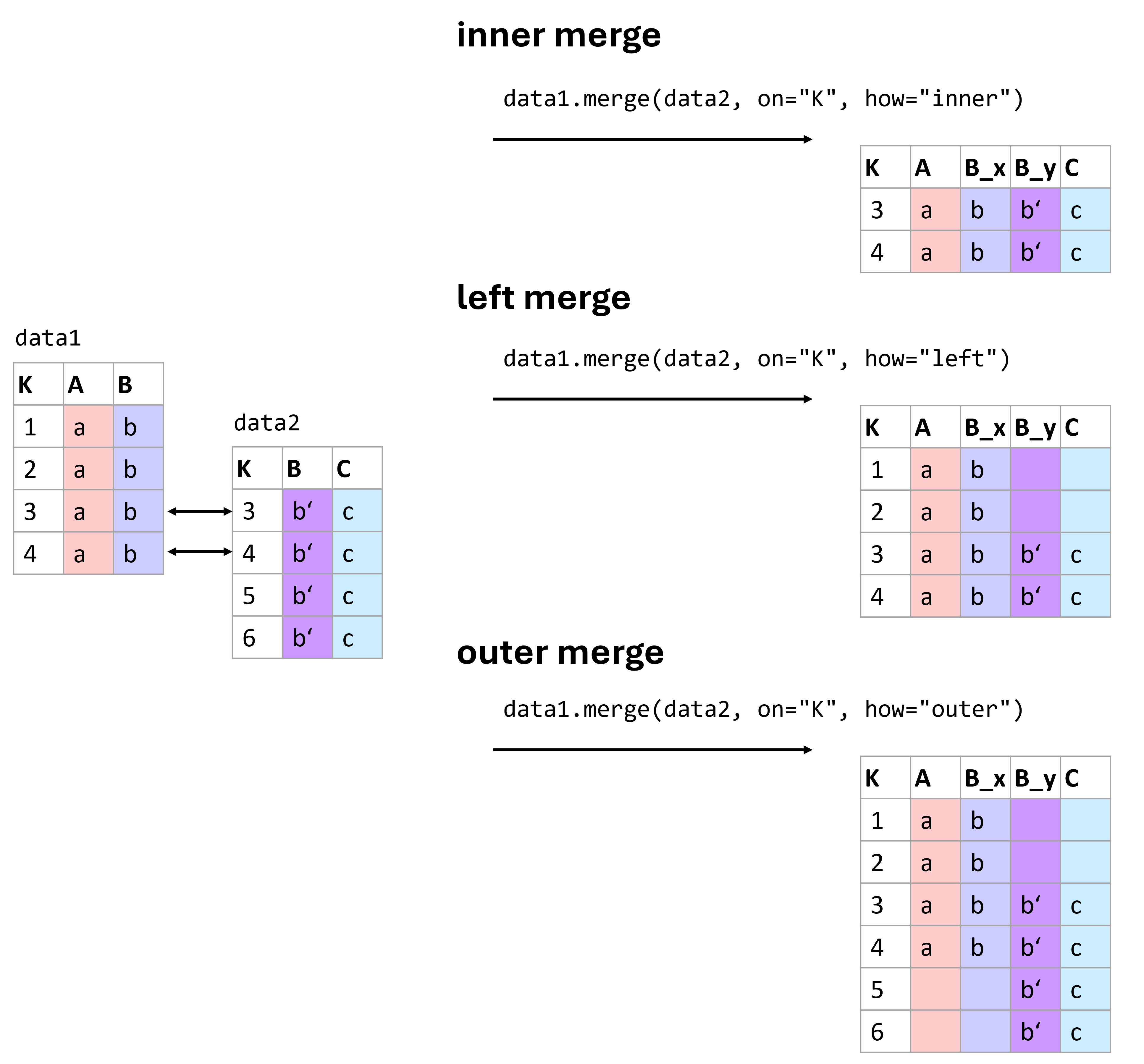
Fig. 9.1 There are different type of merging data. Which one to use is best decided based on the data we have at hand and the types of operations we plan to run with the resulting data. Here are three of the most common types of merges: inner, left, and outer merges.#
Figure (Fig. 9.1) shows some common merging types. More information on different ways to combine data using pandas can be found in the pandas documentation on merging.
9.3.2. Understanding Different Types of Merges#
Combining datasets effectively requires understanding the nature of the relationships between them. This understanding guides the choice of merging technique, each of which can affect the outcome of the analysis differently.
9.3.2.1. Common Types of Merges#
Inner Join
Description: The inner join returns only those records that have matching values in both datasets. This method is most useful when you need to combine records that have a direct correspondence in both sources.
Use Case: Analyzing data where only complete records from both datasets are necessary, such as matching customer demographics with their purchasing records.Outer Join
Types:Full Outer Join: Combines all records from both datasets, filling in missing values with NaNs where no match is found.
Left Outer Join: Includes all records from the left dataset and the matched records from the right dataset.
Right Outer Join: Includes all records from the right dataset and the matched records from the left dataset.
Use Case: Useful when you want to retain all information from one or both datasets, filling gaps with missing values for further analysis.
To illustrate these concepts, let’s see practical examples.
# Create sample data for products
data_products = pd.DataFrame({
    'ProductID': [101, 102, 103, 104],
    'ProductName': ['Widget', 'Gadget', 'DoesWhat', 'DoSomething']
})

# Create sample data for sales
data_sales = pd.DataFrame({
    'ProductID': [101, 102, 104, 105],
    'UnitsSold': [134, 243, 76, 100]
})
data_products.head()
| ProductID | ProductName | |
|---|---|---|
| 0 | 101 | Widget |
| 1 | 102 | Gadget |
| 2 | 103 | DoesWhat |
| 3 | 104 | DoSomething |
data_sales.head()
| ProductID | UnitsSold | |
|---|---|---|
| 0 | 101 | 134 |
| 1 | 102 | 243 |
| 2 | 104 | 76 |
| 3 | 105 | 100 |
Inner Join Example:
inner_join_df = pd.merge(data_products, data_sales, on='ProductID', how='inner')
print("Inner Join Result:")
inner_join_df.head()
Inner Join Result:
| ProductID | ProductName | UnitsSold | |
|---|---|---|---|
| 0 | 101 | Widget | 134 |
| 1 | 102 | Gadget | 243 |
| 2 | 104 | DoSomething | 76 |
Left outer join and full outer join examples:
left_outer_join_df = pd.merge(data_products, data_sales, on='ProductID', how='left')
print("Left Outer Join Result:")
left_outer_join_df.head()
Left Outer Join Result:
| ProductID | ProductName | UnitsSold | |
|---|---|---|---|
| 0 | 101 | Widget | 134.0 |
| 1 | 102 | Gadget | 243.0 |
| 2 | 103 | DoesWhat | NaN |
| 3 | 104 | DoSomething | 76.0 |
full_outer_join_df = pd.merge(data_products, data_sales, on='ProductID', how='outer')
print("Full Outer Join Result:")
full_outer_join_df.head()
Full Outer Join Result:
| ProductID | ProductName | UnitsSold | |
|---|---|---|---|
| 0 | 101 | Widget | 134.0 |
| 1 | 102 | Gadget | 243.0 |
| 2 | 103 | DoesWhat | NaN |
| 3 | 104 | DoSomething | 76.0 |
| 4 | 105 | NaN | 100.0 |
9.3.3. Typical Challenges:#
The given example is fairly simple. In practice, you will often face far more complex situation that often require specific work-arounds. Some very common challenges for merging data are:
Duplicates: Data can have repeated or conflicting entries.
Inconsistent Nomenclature: Consistency in naming conventions can save hours of data wrangling later on. A classic example being different formats of names. “First Name Last Name” versus “Last Name, First Name”.
It is therefore often a good strategy to work with a good identifier system where every datapoint is linked to one specific, unique ID. This can be a number, a hash, a specific code, a filename etc.
9.4. Further Cleaning Steps:#
Unit Conversion: Ensuring data is in consistent units.
Data Standardization: This can be done via Min-Max scaling (often termed “normalization”) or, frequently more effective, by ensuring data has a mean of 0 and a standard deviation of 1.
Non-linear Transformations: Sometimes, linear thinking won’t do. Transformations like logarithms can provide new perspectives on data.
Data Types: Ensuring that numeric values aren’t masquerading as strings can prevent potential analytical blunders (e.g., “12.5” instead of 12.5).
Decimal Delimiters: Confusion between comma and dot can change data meaning, e.g., 12,010 becoming 12.01.
9.5. Data Conversion and Formatting#
9.5.1. Importance of Proper Data Types and Consistent Formatting#
Data types and formatting play a critical role in the accuracy and efficiency of data analysis. Incorrect data types or inconsistent formatting can lead to errors or misinterpretations during data processing. For instance, numeric values stored as strings may not be usable for calculations without conversion, and date strings may be misinterpreted if their format is not uniformly recognized. Ensuring data is correctly typed and formatted is crucial for:
Data Quality: Correct types and formats ensure that the data adheres to the expected standards, improving the overall quality and reliability of the dataset.
Analytical Accuracy: Proper data types are essential for performing accurate mathematical and statistical calculations.
Operational Efficiency: Operations on data, such as sorting and indexing, are more efficient when data types are appropriately set.
9.5.2. Converting Data Types in Pandas#
Pandas provides robust tools for converting data types, which is often necessary when data is imported from different sources and formats.
# Sample data with incorrect data types
data = pd.DataFrame({
    'ProductID': ['001', '002', '003'],
    'Price': ['12.5', '15.0', '20.25'],
    'Date': ['2021-01-01', '2021-01-02', '2021-01-03']
})

# Convert 'ProductID' to integer
data['ProductID'] = data['ProductID'].astype(int)

# Convert 'Price' to float
data['Price'] = data['Price'].replace(',', '.').astype(float)

print("Data after conversion:")
print(data)
Data after conversion:
   ProductID  Price        Date
0          1  12.50  2021-01-01
1          2  15.00  2021-01-02
2          3  20.25  2021-01-03
9.5.3. Formatting Data#
Proper formatting involves converting data into a consistent and usable format. This includes date-time conversion, string manipulation, and handling decimal delimiters.
# Convert 'Date' to datetime format
data['Date'] = pd.to_datetime(data['Date'], format='%Y-%m-%d')
print("Data after formatting Date:")
data.head()
Data after formatting Date:
| ProductID | Price | Date | |
|---|---|---|---|
| 0 | 1 | 12.50 | 2021-01-01 |
| 1 | 2 | 15.00 | 2021-01-02 |
| 2 | 3 | 20.25 | 2021-01-03 |
9.5.3.1. Example: Handling Decimal Delimiters#
This example demonstrates how to handle a common issue where decimal delimiters vary between commas and dots, which can lead to misinterpretation of numerical values.
# Sample data with decimal confusion
sales_data = pd.DataFrame({
    'Region': ['US', 'EU', 'IN'],
    'Sales': ['10,000.50', '8.000,75', '1,000.00']
})

# Correcting decimal delimiters based on region
sales_data['Sales'] = sales_data.apply(
    lambda row: row['Sales'].replace('.', '').replace(',', '.') if row['Region'] == 'EU' else row['Sales'].replace(',', ''),
    axis=1
).astype(float)

print("Corrected Sales Data:")
sales_data.head()
Corrected Sales Data:
| Region | Sales | |
|---|---|---|
| 0 | US | 10000.50 |
| 1 | EU | 8000.75 |
| 2 | IN | 1000.00 |
9.5.3.2. String Manipulation#
Handling strings effectively can also play a crucial part in cleaning data, such as trimming extra spaces, correcting typos, and standardizing text formats. String handling in Pandas mostly works just as in regular Python. By using .str we can access columns in a dataframe and apply specific string methods such as .strip() or .split().
# Sample data with string inconsistencies
customer_data = pd.DataFrame({
    'CustomerName': [' Alice ', 'bob', 'CHARLES']
})

# Standardizing string format: trim, lower case, capitalize
customer_data['CustomerName'] = customer_data['CustomerName'].str.strip().str.lower().str.capitalize()

print("Standardized Customer Names:")
customer_data.head()
Standardized Customer Names:
| CustomerName | |
|---|---|
| 0 | Alice |
| 1 | Bob |
| 2 | Charles |
9.6. Further Cleaning Steps#
9.6.1. Removing Duplicates#
Duplicate entries in a dataset can skew analysis and lead to incorrect conclusions. It’s often important to identify and remove duplicates to ensure data integrity.
# Sample data with duplicate entries
data = pd.DataFrame({
    'CustomerID': [1, 2, 2, 3, 4, 4, 4],
    'Name': ['Alice', 'Bob', 'Bob', 'Charlie', 'Dave', 'Dave', 'Dave'],
    'PurchaseAmount': [250, 150, 150, 300, 400, 400, 400]
})

print("Original Data:")
data.head()
Original Data:
| CustomerID | Name | PurchaseAmount | |
|---|---|---|---|
| 0 | 1 | Alice | 250 |
| 1 | 2 | Bob | 150 |
| 2 | 2 | Bob | 150 |
| 3 | 3 | Charlie | 300 |
| 4 | 4 | Dave | 400 |
# Removing duplicates
data_unique = data.drop_duplicates()
print("Data after Removing Duplicates:")
data_unique.head()
Data after Removing Duplicates:
| CustomerID | Name | PurchaseAmount | |
|---|---|---|---|
| 0 | 1 | Alice | 250 |
| 1 | 2 | Bob | 150 |
| 3 | 3 | Charlie | 300 |
| 4 | 4 | Dave | 400 |
9.6.2. Standardizing Data#
Data standardization involves rescaling the values to a standard, such as having a mean of zero and a standard deviation of one (z-score standardization), or scaling data to a fixed range like 0 to 1 (normalization). This is crucial for many algorithms, including many algorithms in dimensionality reduction, clustering or many machine learning. We will therefore skip this for now, and address this question in later chapters where this processing step becomes crucial.
9.7. Conclusions#
In essence, data acquisition and preparation are the unsung heroes of a successful data science endeavor. By ensuring the foundation is robust and the raw materials are of top quality, you set the stage for analytical brilliance.
From my own experience: It is not uncommon that 80% of the work in a data science project goes into the data acquisition and cleaning.